Visualize patterns of missing values

Years ago, I wrote an article that showed how to visualize patterns of missing data.
During a recent data visualization talk, I discussed the program, which used a small number of SAS IML statements.
An audience member asked whether it is possible to construct the same visualization
by using only Base SAS procedures such as the DATA step and PROC SGPLOT. The answer is yes,
although using the DATA step requires a longer program than using PROC IML.

This article shows how to use only Base SAS procedures to create a heat map that reveals patterns or missing values in data.

A heat map that shows missing-value patterns

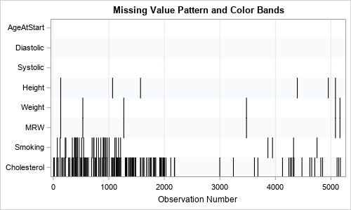
Let’s start by showing the graph we want to create. The graph to the right shows an example for the numerical variables in the Sashelp.heart data.
The black tick marks indicate the missing value in the data. The X axis is the observation number. The Y axis shows the variables in the analysis.

This graph shows the patterns of missing values in the data.
The graph shows that the AgeAtStart, Diastolic, and Systolic variables do not contain any missing values.
The Height, Weight, and MRW variables contain a few missing values, and MRW (which is a measurement of obesity) is missing whenever Weight is missing.
The Smoking and Cholesterol variables contain the most missing values, but primarily for observations early in the data collection process. It looks like some change occurred during the study that improved the collection of nonmissing data for the Smoking and Cholesterol variables.

Some readers might prefer to rotate the plot so that variables become columns and the observation numbers correspond to rows.
That is easily doable, but I prefer to display the categorical variables on the vertical axis.

A DATA step that encodes the missing values

To create this heat map, we need, for each observation number, the names of the variables that contain missing values.
It will save disk space (or RAM) if we store only the observation-variable pairs that contain missing values, not the observation-variable pairs that are nonmissing. (This is called a sparse representation of the missing value pattern.) To detect missing values, I will use the CMISS function in the SAS DATA step. You can pass multiple variables to the CMISS function, and it will return whether any of the variables are missing. If the variables are in a SAS array, then you can use the OF keyword to pass in all variables. For example, if the array is called x, then use the syntax CMISS(of x[*]). You can also loop through the array elements to discover which variables are missing.

A sparse representation stores only the variables and values that are missing. However, it is convenient to use a non-sparse representation for the first and last observations in the data. This ensures that ALL variables appear in the heat map (even those with no missing values), and that the heat map shows the complete range of missing values (1–N) instead of a range that involves only observations that are missing.
Thus, the following program uses a non-sparse representation for the first and last observations.

To make the program general, I define a few macro variables:

• The DSNAME macro variable contains the name of the data set to analyze.
• The NUMERICVARS macro variable contains the name of the variables to analyze. For simplicity, the following statements handle only NUMERIC variables.
  You could extend the program to support character variables. I leave that as an exercise.
• The COLORBANDS macro variable is either 0 or 1. If the macro is 0, then the graph does not display alternating color bands for the discrete axis.
  If the macro is 1, then the graph displays alternating color bands.

/* show how to create a heat map of the missing values for each 
   numeric variable for each observation */
 
%macro VizMissingNumericVar(DSName=,
                            NumericVars=,
                            colorBands=0);
data Heat;
length Variable $32;
set &DSName nobs=numObs;
label obsNum = "Observation Number";
array X[*] &numericVars;
 
/* output all missing/nonmissing for the first and last obs 
   so that X axis ranges over all observation numbers */
if _N_=1 | _N_ = numObs then do;
   /* ensure that the first output value is nonmissing (white) and second is missing (black) */
   obsNum = .; Variable = " "; 
   Value = 0; output;
   Value = 0; output;
   /* ensure that the all variable names are included, in order */
   obsNum = _N_;
   do i = 1 to dim(X);
      Variable = vname(X[i]);
      Value = cmiss(X[i]);
      output;
   end;
end;
/* otherwise, output only the rows and variables that are missing */
else if cmiss(of X[*]) > 0 then do;
   obsNum = _N_;
   do i = 1 to dim(X);
      if cmiss(X[i]) then do;
         Variable = vname(X[i]);
         Value = 1;
         output;
      end;
   end;
end;
keep obsNum Variable Value;
run;
 
proc sgplot data=Heat;
   styleattrs DATACOLORS=(white black);
   heatmapparm x=obsNum y=Variable colorgroup=Value;
   xaxis grid min=0 integer;
   yaxis reverse display=(nolabel)
      %if &colorBands %then %do;
      colorbands=even colorbandsattrs=(transparency=0.8)
      %end;
      ;
run;
%mend;

With this definition, we can call the macro and specify the name of a data set and the name of several numeric variables:

It is helpful to demonstrate new code on a small example that can be easily checked for correctness. The following statements create a small 10-observation data set that contains five numeric variables. The missing value pattern is shown without using alternating color bands:

data Test;
input x1-x5;
datalines;
1 2 3 4 .
. . 3 4 5
1 2 3 4 5
1 2 3 . 5
1 2 3 4 5
. . 3 4 .
1 2 3 4 .
. . 3 4 .
. . 3 4 5
1 2 3 4 .
;
 
ods graphics / width=400px height=150px;
title "Example of Missing Value Pattern";
%VizMissingNumericVar(DSName=Test, NumericVars=x1-x5);

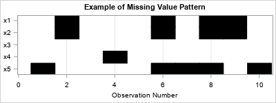
You can inspect the data set and verify that the black cells correspond to the locations of missing values in the data.
Notice that the x1 and x2 variables are missing or nonmissing simultaneously.
The x3 variable is never missing. The x4 variable has only one missing value, whereas half of the x5 values are missing.

The following statements visualize the missing values for the Sashelp.Heart data.
The resulting heat map was shown and discussed at the beginning of this article.

ods graphics / width=500px height=300px;
title "Missing Value Pattern and Color Bands";
%VizMissingNumericVar(DSName = Sashelp.Heart,  
         NumericVars = AgeAtStart Diastolic Systolic 
                      Height Weight MRW Smoking Cholesterol,
         ColorBands=1);

Summary

This article shows how to use Base SAS procedures to visualize the missing-value patterns for numerical variables in a SAS data set. This implementation uses the DATA step and the CMISS function. With additional work, you can extend the program to the case of analyzing either numerical variable, character variables, or both types in a single graph. I leave the details to the motivated reader.