Cohen’s D statistic in SAS

What is Cohen’s d statistic and how is it used? How can you compute it in SAS? This article gives some history behind Cohen’s d statistic.
It shows how to compute the statistic in SAS for the difference in means between two independent samples.
It shows how to estimate a standard error for Cohen’s d statistic.

What is Cohen’s d statistic?

Cohen (1962) performed a meta-analysis on a set of 70 published studies in a psychology journal and examined
the probability of Type-II errors (false negatives) in those studies.
A Type-II error occurs when a study fails to reject the null hypothesis
when it is in fact false. For example, in a two-sample t test, the null hypothesis is that the
mean of two groups are the same. If the mean of the two groups are in fact different, a Type-II
error occurs when a study cannot detect the difference, and the researcher erroneously concludes that the
group means are the same.
Cohen pointed out that Type-II errors are likely to occur when a study is underpowered, meaning that the
sample size is too small to detect the difference. If β is the probability of making a Type-II error, then 1 – β is the power of the test.

In his review, some studies used t tests, some used F tests, some used chi-square tests, and so on. For each kind of test,
Cohen estimated the power of the test.
In order to compare different studies, he introduced a way to standardize the results of the studies.

The main source for this blog post is
Goulet-Pelletiera and Cousineau (2018), which is an excellent resource that discusses the equations for the d statistic, the standard error, and confidence intervals.
For a shorter overview, there is
a Wikipedia article that discusses several standardized statistics related to Cohen’s d.

Cohen’s d for two independent samples

For the t tests of two independent samples, Cohen created a standardized statistic,
called Cohen’s d statistic, which is


     d = (m1 – m2) / s_p


where m1 is the mean of the first group, m2 is the mean of the second group, and s_p is the pooled standard deviation of the measurements.
The pooled standard deviation is the square root of the pooled variance, which is


\(
s_p^2 = \frac{(n_1-1)s_1^2 + (n_2-1)s_2^2}{n_1 + n_2 – 2}
\)


where n_i and s_i² are the size and variance of the i_th group.
By using the pooled standard deviation, we are assuming that the variances in the two populations are equal.
Cohen’s d also assumes that the distribution of each population is normal.

Cohen’s d statistic is sometimes called the standardized mean difference (SMD).
The remainder of this article shows how to compute Cohen’s d statistic in SAS for a two-sample independent (unpaired) t test.

The Wikipedia article on Cohen’s d statistic mentions that the d statistic is often used to estimate the sample size that you need
in a study to detect a true difference. When d is small, you need large samples to reject the hull hypothesis of no difference.
Notice that a small d can mean that the group means are close to each other, or that the pooled variance is large relative to the difference.

There are no universal rules for interpreting Cohen’s d, but
in Cohen’s original paper (Cohen (1962), Table 2, p. 147),
he proposes the following rule of thumb:

• An mean difference is “small” if |d| ≈ 0.25
• An mean difference is “medium” if |d| ≈ 0.5
• An mean difference is “large” if |d| ≈ 1 or more

Cohen’s d is a biased statistic

Cphen’s d is a biased statistic. It overestimates the effect size in the population.
Hedges (1981) developed a factor (less than 1) that eliminates the bias by shrinking Cohen’s d. The unbiased result
is called Hedges’ g. It is defined by g = J(ν)*d, where J(ν) is a factor that depends on the sample sizes:


\(
J(\nu) = \frac{\Gamma(\nu)}{\sqrt{\nu/2}\, \Gamma((\nu-1)/2)}
\)


where ν = n1 + n2 – 2 is the degrees of freedom and Γ is the Gamma function.
Goulet-Pelletier and Cousineau (2018, p. 245) state, “As a rule of thumb, unbiased estimates
should always be used and consequently, Hedges’ g should always be preferred over Cohen’s d.”

Cohen’s d from PROC TTEST

In SAS, you can use PROC TTEST to compute
Cohen’s d and Hedges’ g. Let’s run an example. The documentation of PROC TTEST
includes a data set about golf scores for males and females in a physical education course. The research question is whether there
is a difference in the mean golf scores based on the gender of the students:

/* Golf scores for students in a physical education class (modified from PROC TTEST documentation) */
data scores;
input Gender $ Score @@;
datalines;
f 75  f 76  f 80  f 77  f 80  f 77  f 73
m 82  m 80  m 85  m 81  m 78  m 83  m 82 m 76 m 81
;
/* run t test for two independent samples */
proc ttest data=scores plots=none;
   class Gender;
   var Score;
   ods select Statistics;
   ods output Statistics=TTestOut;
run;

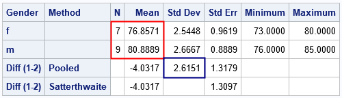
I overlaid a few rectangles on the output to highlight the statistics that are used to create Cohen’s d.
The red rectangle shows the sample sizes (n1 and n2) and the means (m1 and m2) for each group.
The blue rectangle shows the pooled standard deviation. The ODS OUTPUT statement writes that table to a SAS
data set. The interpretation is that the average golf score for a male in the class is about 4 strokes less than for the females.

If you want to compare male and female differences across several sports (such as bowling and weightlifting),
you cannot use the raw scores. Four strokes in golf does not equate to four pins in bowling or four kilos in weightlifting.
You can compare the standardized mean differences by dividing the raw differences by the (pooled) standard deviation.
This is what Cohen’s d does.
The following DATA step reads in the statistics for each group and forms the Cohen’s d and Hedges’ g statistics:

data EffectSize;
retain n1 m1 n2 m2 PooledSD;
keep n1 m1 n2 m2 PooledSD d g J;
label d="Cohen's d" g="Hedges' g" J="Hedges' correction factor";
set TTestOut end=EOF;
if _N_=1 then do;       /* read 1st row */
   n1 = N; m1 = Mean;
end;
if _N_=2 then do;       /* read 2nd row */
   n2 = N; m2 = Mean;
end;
if _N_=3 then          /* read 3rd row */
   PooledSD = StdDev;
if EOF then do;
   /* form Cohen's d, which is a biased estimator */
   d = (m1 - m2) / PooledSD;   
   /* J is Hedge's correction factor. See Cousineau & Goulet-Pelletier (2020, p. 244) */
   df = n1 + n2 - 2;
   J =  exp( lgamma(df/2) - lgamma((df-1)/2) - log(sqrt(df/2)) ); 
   g = J * d;                  /* Hedge's g, which is an unbiased estimator */
   output;
end;
run;
 
proc print label noobs data=EffectSize;
run;

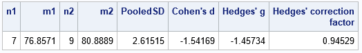
The value for Cohen’s d is about -1.54.
As expected, Hedges’ g (-1.45) is a little smaller in magnitude.
You can interpret this value of Cohen’s d in two ways:

• According to Cohen’s rule-of-thumb, a value of |d| > 1 is a “large difference.”
• The “standardized unit” for the golf scores is based on the pooled standard deviation, which is 2.6 strokes.
  Cohen’s d tells us that the mean male score is about -1.54 standardized units less than the mean female score

One comment on the computation of the J correction factor. The factor contains a ratio of gamma functions, which grow very quickly.
When you compute a ratio like R=A/B, where A and B can be large, it is better to compute it as R=exp(log(A/B)).
That enables you to compute the ratio on the log scale as log(A) – log(B). In SAS, the LGAMMA function computes the
log of the gamma function.

The standard error of Cohen’s d

For small sample sizes, we should always question the precision of a point estimate.
That is the purpose of the standard error. A small standard error indicates that the
point estimate is precise, whereas a large standard errors indicates less precision.

Goulet-Pelletier and Cousineau (2018) publish a table (Table 3, p. 246) that contains seven different
estimates of the variance of Cohen’s d or Hedges’ g!
The formulas include a generic symbol, δ, for the effect size in the population.
If you are using Cohen’s d, substitute δ=d into the formulas.
If you are using Hedges’ g, substitute δ=g into the formulas.
Because
different sources will use different formulas, you should clarify which formula is being used
when someone reports “the” standard error.

The best formula is the “true formula” by Hedges (1981, eq, 6b), which includes the correction factor, J(ν),
which requires using the Gamma function.
In the era of modern computer power, there is no reason to use any other formula.
The other formulas are approximations.
However, the approximations are often presented in papers and textbooks.
For the sake of completion, I will include two of the most popular approximations,
the Hedges approximation (Hedges, 1981) and the MLE approximation (Hedges and Olkin, 1985).
The formulas are in Table 3 of Goulet-Pelletier and Cousineau (2018), or you can look directly at the SAS code.

The following DATA step reads in the previous data set, which has the values n1, n2, d, and g.
It uses these statistics to estimate the standard error for both d and g:

/* The formulas for standard errors are from Table 3 on p. 246 of
   Goulet-Pelletiera and Cousineau (2018) https://www.tqmp.org/RegularArticles/vol14-4/p242/p242.pdf 
   The formulas are in terms of delta, which is the population standardized effect size. 
   Plug in d or g for delta.  The best estimate of SE is "True SE". 
 
   Var     Label               Reference
   ======  ===========         =================
   SE      "True SE"           Hedges (1981), p. 111, Eqn. 6b 
   SE_mle  "MLE Approx SE"     Hedges & Olkin (1985)
   SE_h    "Hedges' Approx SE" Hedges (1981, p. 117) approx for N > 50
*/
data SEEffectSize;
length Statistic $10;
keep Statistic Estimate SE SE_mle SE_h;
label Estimate="Estimate" SE="True SE" SE_mle="MLE Approx SE" SE_h="Hedges' Approx SE";
set EffectSize;
do i = 1 to 2;
   if i=1 then do;
      Statistic="Hedges' g"; Estimate = g;    /* g is a better estimate of effect size */
   end;
   else do;
      Statistic="Cohen's d"; Estimate = d;    /* but you can use d, if you want */
   end;
 
   /* the harmonic mean of n1 and n2 is  2*n1*n2/(n1+n2) */
   delta = Estimate;          /* use either d or g as the estimate */
   w = 2/harmean(n1,n2);      /* 2/H(n1,n2) = (n1+n2)/(n1*n2) */
   df = n1 + n2 - 2;          /* degrees of freedom */
   /* The best estimate of standard error is the "true formula" */
   var = df/(df-2) * (w + delta**2) - (delta/J)**2;
   SE = sqrt( var );           
 
   /* Hedges' Approx SE: Hedges (1981, p. 117) approx for N > 50 */
   var_h = w + delta**2/(2*df);   
   SE_h   = sqrt( var_h );
   /* MLE Approx SE: Hedges & Olkin (1985), Eqn.11, p.82.
      This is used in the Handbook of Research Synthesis (p. 238)
      https://stats.stackexchange.com/questions/8487/how-do-you-calculate-confidence-intervals-for-cohens-d */
   factor = (df+2)/df;       /* MLE correction factor */
   SE_mle = sqrt( var_h * factor );
   output;
end;
run;
 
proc print label noobs data=SEEffectSize;
run;

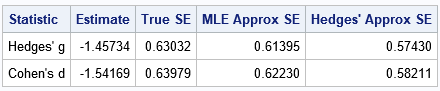
The standard errors are relatively large compared to the point estimates. If you were to collect data on a new set of student golf scores,
it would not be surprising to obtain a new value of Hedges’ d that is larger or smaller by 0.63 or more. A more precise statement
would use confidence intervals, which I will postpone for another article.

Summary

This article focuses on Cohen’s d statistic for the important case of two independent samples. (There are other versions of Cohen’s d; see Wikipedia.)
You can think of Cohen’s d statistic as a standardized mean difference. When d is small, the effect will be hard to detect unless you have a large sample.
Cohen’s d is biased, so you should use Hedges’ g, which adjusts for the bias. For either statistic, you can compute the standard error of the
statistic by using a “true formula,” although some papers and textbooks use an approximation to the standard error.
This article implements all formulas in SAS by using PROC TTEST and the DATA step.

References

• 
  Goulet-Pelletier, J-C, and Cousineau, D. (2018) “A review of effect sizes and their confidence intervals, Part I: The Cohen’s d family.” The Quantitative Methods for Psychology 14.4: 242-265.
• 
  Hedges, L. V. (1981) “Distribution theory for Glass’s estimator of effect size and related estimators.” Journal of Educational Statistics, 6(2), 107–128.
• 
  Hedges, L. V., & Olkin, I. (1985). Statistical methods for
  meta-analysis. San Diego, CA: Academic Press.