The sample median is a biased estimator for skewed distributions

Did you know that,
for skewed distributions, the sample median is a biased estimator of the population median?
You can show this in two ways. For any distribution, you can run a Monte Carlo simulation that
reveals the bias. And, for some distributions (such as the exponential distribution), you can explicitly write a formula
for the expected value of the sample median. The formula proves that the sample median is a biased estimate, and
it reveals the size of the bias.

Is bias a big deal?

For data analysis tasks, I don’t often worry about biased statistics.
Bias is defined as the difference between the expected value of an estimator and the population parameter.
For most statistics,
the standard error of the statistic is much larger than its bias, thus
bias isn’t very important in practice.
Furthermore, many statistics are asymptotically unbiased, so the bias is small for large samples.

However, knowing whether a statistic is biased is important for Monte Carlo simulation studies.
In a simulation study, you know the exact value of a population parameter.
When I develop a simulation, I often verify its correctness by
running many simulations and checking that the Monte Carlo estimate converges to the population parameter.
However, a biased statistic does not converge to the population parameter! The Monte Carlo estimate converges to the
expected value of the statistic. For a biased estimator, the expected value is different from the population parameter,
by definition.
As the number of Monte Carlo iterations (B) increases, the standard error of the simulation shrinks toward zero, but the bias remains constant.

The median of an exponential distribution

I recently wrote an article about the convergence of Monte Carlo estimates.
The example in that article studied the sample mean for random samples drawn from an exponential distribution
that has a scale parameter (λ) with the value 10.
You can look up in Wikipedia or a textbook that the median of the exponential distribution is
log(2)*λ. So, when λ=10, the median of the Expo(10) distribution is 6.9315.

In the previous article, the sample size was N=100.
This article uses N=99 instead. Since the sample median is the “middle value” in the sample,
using an odd sample size makes the theoretical formulas a little easier to understand.

A Monte Carlo simulation for the median

To demonstrate that the sample median is a biased statistic, let’s run the following Monte Carlo simulation:

• Choose B=10,000 as the number of simulations.
• Draw B random samples of size N=99 from an Expo(λ=10) distribution.
• For each random sample, compute the sample median.
• Average the sample statistics to obtain the Monte Carlo estimate of the population median.
• Compare the Monte Carlo estimate to the known value of the distribution’s median. The difference is the bias of the sample median in samples of size 99.

/* Monte Carlo simulation for median of EXPO(10) distribution. Estimate bias in the 
   sample median for samples of size N=99.
   The true median is log(2)*lambda ~ 6.93147. */
proc iml;
lambda = 10;                   /* generate random sample of size N from Expo(lambda) */
expo_median = log(2)*lambda;
 
call randseed(12345);
N = 99;                        /* sample size is odd ==> median is middle order statistic */
B = 10000;                     /* number of Monte Carlo samples */
 
sample_median = j(B,1,.);
x = j(N,1);
do i = 1 to B;
   call randgen(x, "Expo", lambda);
   sample_median[i] = median(x);
end;
 
MC_est = mean(sample_median);
MC_SE_est = std(sample_median) / sqrt(B); /* std error for Monte Carlo estimate */
width = 3*MC_SE_est;                      /* 3*SE ==> 99.7% CI */
Lower_CL = MC_est - width;
Upper_CL = MC_est + width;
print MC_est expo_median (MC_est-expo_median)[L="Est Bias"];
print MC_est MC_SE_est width Lower_CL Upper_CL;

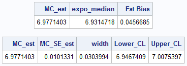
The simulation shows two facts.
First, the Monte Carlo estimate is larger than the median of the distribution. The estimated bias is approximately 0.0457.
Is that bias large? Well,
“large” or “small” must be compared to some standard unit, and for a statistic the “unit” is the standard error of the statistic.
The asymptotic standard error of the median statistic is approximately λ/sqrt(N) ~ 1.005.
So, the bias is less than 5% of the standard error. In other words, if you are analyzing one single data set of size N=99, the
standard error of the median is 20 times larger than the bias. This is why we typically can ignore bias.

The second fact is the accuracy of the Monte Carlo estimate. After 10,000 simulations, a
99.7% confidence interval for the estimate has a half-width of 0.03. We are fairly confident that the expected value of the
sample median is within 0.03 of the computed Monte Carlo estimate.
The next section shows that the expected value for the sample median is 6.982, which is indeed inside the confidence interval for this set of random trials.

Order statistics for the exponential distribution

For the exponential distribution, you can use order statistics to explicitly compute the expected value of the sample median.
To simplify matters, let’s assume that N=2*k – 1 is an odd number.
To simplify notation, let’s sort the data and denote the values by


X₁ ≤ X₂ ≤ …≤ X_k ≤ …≤ X_N.

The median is the “k_th order statistic,” which is simply the k_th element in the sorted list of values.
As shown in a Wikipedia article on order statistics,
the expected value of the k-th smallest observation is known to be:


E[X_k] = λ ∑_i=1^k 1 / (N – i + 1)

For N=99, k=50. The following SAS IML function evaluates the expected value of the sample median for an Expo(10) sample:

proc iml;
/* For a sample of size N drawn from an Expo distribution,
   the expected value of the k_th smallest obs (the k_th order statistic)
   is given by an explicit formula. 
*/
start EExpOrderStat(k, N, lambda=1);
   i = T(1:k);
   return( lambda * sum( 1 / (N - i + 1) ) );
finish;
 
N = 99;
lambda = 10;
/* expected value of the median for an ODD sample ~ Expo(lambda) */
k = (N+1)/2;
Emedian_N99 = EExpOrderStat(k, N, lambda);
print Emedian_N99;

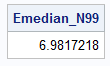
The expected value is 6.98172. Notice that this value is inside the 99.7% confidence interval from our Monte Carlo simulation.

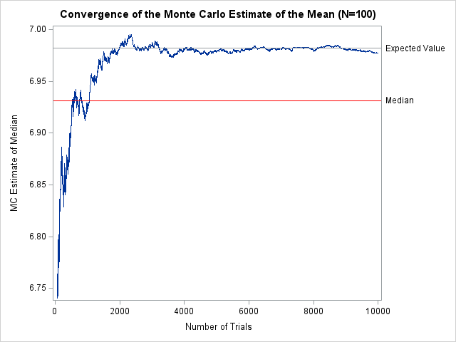
Convergence of a biased statistic

What does the convergence look like if you graph it?
You will see an estimate that converges, but not to the parameter value. Instead, it converges to the expected value of the statistic.
The following graph shows the Monte Carlo estimate of the sample median after k simulations, k=1..B.
You can see that the estimate converges, but there is a big gap (the bias) between the estimate and the population parameter.

Conclusion

For symmetric distributions,
the sample median is an unbiased estimator of the population median.
Furthermore, the estimator is asymptotically unbiased, which means the bias is negligible for very large samples.
However, for right-skewed distributions like the exponential distribution, the sample median is biased upwards.
This bias is important for Monte Carlo simulations because the Monte Carlo estimate converges to the expected value
of a statistic. When the statistic is biased, the Monte Carlo estimate converges to a value that is different from
the population parameter. This is most apparent when you are simulating small samples.

Appendix: The standard error of the median for an exponential distribution

In the text, I claimed that the asymptotic standard error of the sample median of Expo(λ) data is
approximately λ/sqrt(N). But wait, isn’t that the well-known formula for the standard error of the mean? We want the standard error of the median!

The formula is correct. The formula relies on the fact that the sampling distribution of the median is asymptotically normal for continuous distributions.
This asymptotic normality is true for all percentiles. It is the basis for the CIPCTLNORMAL option in PROC UNIVARIATE,
which provides confidence intervals, assuming the sampling distribution of the percentiles are normal.
If you like math, you can read the proof in these lecture notes from McGill University.

Asymptotically, the distribution of the sample median is normally distributed with standard error


SE_med = 1 / (2*sqrt(N)*f(M))


where f is the PDF of the continuous distribution and M is the true population median.
(Obvious, we need f(M) ≠ 0.)
For the exponential distribution,
f(x) = (1/λ) exp(-x/λ) and M = λ*log(2).
Thus, a several terms cancel and


f(M) = 1/(2λ)

Consequently, the asymptotic standard error is SE_med = λ/sqrt(N), which is the same formula as the standard error of the mean.