In general, it is very difficult to compute a probability for a multivariate continuous distribution.
For all continuous distributions, the probability requires solving a complicated multiple integral.
For example, the probability for a bivariate normal distribution requires integrating the bivariate normal density
over a two-dimensional (2-D) area.
The probability for a k-dimensional distribution requires integrating the density over a k-D volume.
The probability depends on the density (PDF) of the distribution as well as the region of integration.
One special region is the orthant. An orthant is a generalization of a quadrant.
In two dimensions, the Cartesian coordinate system divides the plane into four quadrants.
In three dimensions, the Cartesian coordinate system divides the plane into eight octants.
In k dimensions, there are 2k orthants.
It is rare to find an exact formula for the probability of a multivariate distribution.
Amazingly, there are formulas for the probability of a standardized multivariate normal (MVN) distribution in an orthant
(Genz and Bretz (2009) p. 11-13, who cite Sheppard (1898), D. R. Childs (1967), and H. J. Sun (1988)).
This article shows the formulas for dimensions 1, 2, and 3. In a subsequent article, I will discuss
a SAS IML function that implements a formula for dimension k=4.
The general case was solved by Childs (1967) and extended by Sun (1988), so
I refer to these formulas as the Childs-Sun formulas.
As shown in a previous article, it suffices to compute a probability for the standardized MVN distribution
because a probability for a general MVN distribution can always be found by standardizing the problem.
To save typing, this article deals exclusively with the standardized MVN distribution and often omits the word “standardized”.
Orthant probabilities
For a vector X, the signs of X are constant within each orthant.
For example, a 2-D vector has signs (+1, +1) when it is in the first quadrant, and signs (-1, -1) when it is in the third quadrant.
The term “orthant probability” traditionally refers to the first orthant, where all signs are positive.
The MVN distribution is symmetric under the transformation X → -X, so the probability that X~MVN(0,R) is in the “all-signs-positive” octant
equals the probability that X is in the “all-signs-negative” octant.
The “all-signs-negative” octant is important in probability and statistics.
It represents the “CDF region,” which is a left-tail probability. For example, for a 2-D random vector X=(X1,X2), the CDF
evaluated at (0,0) is Φ2(0,0) = P(X1<0 and X2<0), which is the probability that X is in the third quadrant. In terms of an integral,
\(
\Phi_2(0,0; \rho)
=
\int_{-\infty}^{0} \int_{-\infty}^{0} \phi_2(x_1, x_2; \rho)\, dx_2 \, dx_1
\)
Here, ρ is the Pearson correlation between X1 and X2, φ2 is the bivariate standard normal density,
and Φ2 is the bivariate standard normal CDF.
This concept generalizes to higher-dimensional distributions: the “CDF orthant” is the “all-signs-negative” orthant for which every coordinate of X has a negative sign.
The CDF of the standardized normal distribution at the origin is the integral of the distribution’s density over that orthant.
This article shows some Childs-Sun formulas for these probabilities for a general correlation matrix.
Orthant probabilities in dimensions 1 and 2
For the one-dimensional problem, the 1-D orthant is the set {X < 0}.
The CDF at zero is P1 = Φ1(0) = 0.5. You can obtain this value by solving an integration problem, but it is also evident from
the fact that the normal distribution is symmetric about 0.
For this article, the important fact is that there is a formula for the 1-D orthant probability: P1 = 1/2.
For 2-D, the correlation matrix has one parameter, ρ = R[1,2], which is the correlation between the bivariate normal variates X1 and X2.
The 2-D (bivariate) formula (originally found by Sheppard, 1898) is
\(P_2 = \Phi_2(0,0; \rho) = \frac{1}{4} + \frac{1}{2\pi} \sin^{-1}(\rho)\)
Let’s run a simple DATA step to verify this result. In SAS, you can use the PROBBNRM function to compute a bivariate normal probability:
/* 2-D orthant probability for various rho values */ data MVN2D; input rho @@; pi = constant('pi'); P2_formula = 1/4 + 1/(2*pi) * arsin(rho); P2_integral = probbnrm(0, 0, rho); diff = P2_formula - P2_integral; drop pi; datalines; -0.8 -0.5 0 0.5 0.8 ; proc print data=MVN2D noobs; run; |
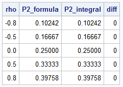
As shown in the output, the formula agrees with the PROBBNRM function to within machine precision.
Orthant probabilities in dimension 3
In 3-D the standard multivariate normal distribution has three parameters: the off-diagonal elements of the 3×3 correlation matrix, R.
The formula for the orthant probability in dimension 3 is given by
\(P_3 = \frac{1}{8} + \frac{1}{4\pi} \left( \sin^{-1}(R_{12}) + \sin^{-1}(R_{13}) + \sin^{-1}(R_{23}) \right)
\)
Notice that you can write P3 by using a summation formula in which you sum over the indices
of the upper triangular elements of the correlation matrix, R.
To validate this formula, let’s use a Monte Carlo estimation routine, which was developed in a previous article. The following SAS IML program
evaluates the formula for a few correlation matrices, and compares the formula and the Monte Carlo estimate.
/* 3-D orthant probability for various correlation matrices, R */ proc iml; /* Use Monte Carlo simulation to estimate the probability that a MVN random variable is less than a specified value in each coordinate. See https://blogs.sas.com/content/iml/2026/05/04/standardize-mvn-probabilities.html The function estimates CDF(b). */ start MC_CDFMVN(N, b, Sigma, mu=j(1,ncol(Sigma),0)); X = randnormal(N, mu, Sigma); inRegion = j(N, 1, 1); do i = 1 to ncol(b); v = (X[,i] < b[i]); /* binary variable for the i_th coordinate */ inRegion = inRegion & v; /* find the intersection of all conditions */ end; return mean(inRegion); /* proportion of random points that satisfy criterion */ finish; /* Evaluate the MVN CDF at the origin (="orthant probability") by using the exact P3 formula */ start Orthant_P3(R); pi = constant("pi"); upper_tri_corrs = R[ {2 3 6} ]; sum_arsin = sum( arsin( upper_tri_corrs ) ); prob = 1/8 + sum_arsin / (4 * pi); return(prob); finish; N = 1E6; /* size of Monte Carlo sample */ b = {0 0 0}; /* the origin */ call randseed(1234); /* Example 1: AR(1) correlation matrix */ R = {1 0.5 0.25, 0.5 1 0.5, 0.25 0.5 1 }; P3_formula = Orthant_P3(R); P3_MC_est = MC_CDFMVN(N, b, R); diff = P3_formula - P3_MC_est; print P3_formula P3_MC_est diff; /* Example 2: positive and negative correlations */ R = {1 -0.5 -0.1, -0.5 1 0.8, -0.1 0.8 1 }; P3_formula = Orthant_P3(R); P3_MC_est = MC_CDFMVN(N, b, R); diff = P3_formula - P3_MC_est; print P3_formula P3_MC_est diff; |
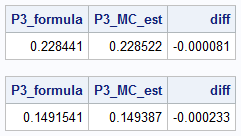
Results are shown for two different correlation matrices. The formula in the Orthant_P3 function is exact.
The Monte Carlo estimate is close to the exact value.
The computation for other 2-D quadrants
The formula is more powerful than it initially seems because of reflective symmetries of the multivariate normal distribution.
The Childs-Sun formula enables you to compute the probability in all orthants, not just the “CDF orthant” where
every component of the random variable has a negative sign. This is because you can change the signs of the components of the
MVN random variable to obtain the other quadrants. Geometrically, “changing the sign” means considering the transformation
Xi → -Xi for some coordinate. This transformation changes the sign of the correlation
between Xi and the other variables. Thus, you can obtain the correlation matrix for any transformation that reflects
one or more coordinates.
Let’s see how this works in two dimensions.
Let ρ be the off-diagonal (R[1,2]) correlation. Here is how to get the probability in all four quadrants:
- Quadrant I: This is the orthant probability, P2 = 1/4 + arsin(ρ) / (2π).
- Quadrant II: To find the probability in the region Q2 = {X1 < 0, X2 > 0},
define Y1 = -X1 and Y2 = X2. Y is bivariate normal with correlation -ρ. Because arsin(-ρ) = -arsin(ρ),
the probability in Q2 is 1/4 – arsin(ρ) / (2π). - Quadrant III: To find the probability in the region Q3 = {X1 < 0, X2 < 0},
define Y1 = -X1 and Y2 = -X2. Y is bivariate normal with correlation ρ, so the probability over Q3 is P2. - Quadrant IV: To find the probability in the region Q4 = {X1 > 0, X2 < 0},
define Y1 = X1 and Y2 = -X2. Y is bivariate normal with correlation -ρ, therefore
the probability in Q4 is 1/4 – arsin(ρ) / (2π).
The computation for other k-D orthants
The same idea applies for any dimension.
The Childs-Sun formula gives the orthant probability in the first quadrant where all coordinates are positive.
Every orthant is identified by a sign vector s=(s1, s2, …, sk), where each component is either +1 or -1.
To compute the probability that X~MVN(0, R) is in the orthant with the sign vector s, do the following:
- Define a new MVN variable, Y = (s1*X1, s2*X2, …, sk*Xk).
- Compute the correlation matrix for Y. This requires changing some of the signs of the off-diagonal elements in R. See the Appendix for details.
- Use the Childs-Sun formula to find the probability that Y is in the first orthant. This is also the
probability that X is in the orthant with sign vector s.
Summary
In summary, this article shows three Childs-Sunformulas for computing the orthant probability for a
standardized multivariate normal distribution
with correlation matrix R in dimension k:
- If k=1, the univariate probability is \(P_1 = \frac{1}{2}\).
- If k=2, the bivariate probability is \(P_2 = \frac{1}{4} + \frac{1}{2\pi} \sin^{-1}(R_{12})\).
- If k=3, the trivariate probability is
\(P_3 = \frac{1}{8} + \frac{1}{4\pi} \left( \sin^{-1}(R_{12}) + \sin^{-1}(R_{13}) + \sin^{-1}(R_{23}) \right)\)
You can apply these formulas as written to compute the probability in the first orthant (all signs positive) or in the “CDF orthant” (all signs negative). You can use the reflective symmetry of the MVN distribution to find the probabilities in every other orthant.
Appendix: How the correlation matrix changes under coordinate reflections
This main article indicates that you can apply reflection transformations for coordinates of X~MVN(0,R) and find a
new correlation matrix, C, such that Childs-Sun formula applies to C gives the probability that X is in some orthant.
This appendix shows the linear algebra steps.
Suppose X~MVN(0,R), and you want to find the probability that X is in an orthant defined by a sign vector s=(s1, s2, …, sk). In this vector, each si is either +1 or -1.
We can use s to define a new random vector, Y, such that Y is in the first orthant exactly when X is in the target orthant.
Let S be the k x k diagonal matrix whose diagonal elements are the components of the sign vector, s.
Define the linear transformation Y = S X.
Because S is a diagonal matrix of signs, the i_th component of Y is simply Yi = si * Xi.
By definition, if X is in the target orthant, then the sign of Xi matches si.
Therefore, the product si * Xi is always positive, which means Y is in the first orthant.
Because Y is a linear transformation of MVN variables, it is also multivariate normal.
The expected value of Y is E[Y] = S E[X] = 0.
The covariance matrix for Y (call it C) is given by the standard formula for the variance of a linear transformation:
\(
C = \text{Cov}(Y) = S \text{Cov}(X) S^T = S R S
\)
If you multiply the matrices, you will find that the elements of C are given by
Cij = si sj Rij.
Because si2 = 1, the diagonal elements of C are 1, which means C is a valid correlation matrix.
The off-diagonal elements of C simply flip the sign of the correlation whenever exactly one of the two corresponding variables is reflected.
In summary, Y~MVN(0, C). The Childs-Sun formula with the correlation matrix C
gives the probability that Y is in the first orthant.
This is exactly the probability that X is in the orthant with the given sign vector, s.