Levy flight and vectorizing a simulation in SAS

A previous article shows a simulation of two different models of a foraging animal.
The first model is a random walk, which assumes that the animal chooses a random direction, then takes a step that is distributed according to a Gaussian random variable.
In the second model, the animal again chooses a random direction, but the distance it travels is distributed randomly according to a heavy-tailed distribution.
The difference is dramatic: the Gaussian random walk stays close to the initial position, whereas in the
Levy-flight model, the animal forages a few times in one area, then takes a long trip to a second are, where it forages again.
Biologists use the second model for many animals that hunt at sea, including albatross, sharks, turtles, penguins, and tuna.

My previous article used the SAS DATA step to simulate each model. Recently, my colleague, Jay Laramore, wrote a simulation of Levy flight by using the SAS IML language.
Jay used a different parameterization than I did, but I was able to modify his program to show how to
convert my previous DATA step simulation into the IML language.

This article emphasizes several important ideas about statistical programming in the SAS IML language:

• 
  It is easy to create user-defined functions in the IML language. Therefore, you can break up a simulation into independent components
  that can be independently written, tested, and debugged.
• 
  By using the components in a simulation, you can easily see the similarities and difference between two different methods.
• 
  Often, you can write a simulation in SAS IML that is vectorized for performance.
• 
  The IML language is built for high-dimensional computations, so it is easy to implement random walks in higher dimensions.

Gaussian versus heavy-tailed steps

The previous article showed how to use Base SAS functions and macros to generate the random numbers that are used to move
from one position to the next. A Gaussian distribution has a “light tail.” For example, we know from the famous 68-95-99.7 rule for normal distributions
that 99.7% of random observations are less than three standard deviations from the mean. For example, if you generate distances according to the
magnitude of N(0, σ) variates, then you would expect 99.7% of the distances to be less than 3σ units in length.
In this article, the distances follow the folded normal distribution, but the light tail remains.

In contrast, the Levy distribution has a heavy tail. Therefore,
the probability of an extreme distance is much greater. In fact, a random variate from the Levy distribution
might be larger than the distance that a real animal can swim/fly/run in one time period.
Therefore, biologists are forced to truncate extreme distances
to conform with physical realities. This leads to the truncated Levy distribution.

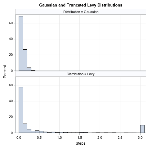
The graph to right compares 1,000 random distances generated from each distribution. The top histogram is from the (folded) N(0, 0.1) distribution. As expected,
few distances exceed three standard deviations or 0.3. The bottom histogram shows random distances from the
Levy(0, 0.3) distribution. Any variates greater than 3 are replaced with 3, which is the longest distance that this animal can travel in one time unit.
Although the probability that the animal will take a small step is similar in both graphs, the animal is unlikely to take a large step in the first model,
whereas a large step is
moderately likely in the second model.

Simulate Gaussian walks and Levy flights in SAS IML

The SAS IML language enables you to define functions that can be independently tested. You can then assemble the functions to perform
algorithms. To simulate a random walk or flight, you can define the following functions:

• Generate a random step: You might define a function (RandAbsNormal) that simulates from the (folded) normal distribution, and another function (RandTruncLevy) that simulates from a truncated Levy distribution.
• Generate a direction uniformly at random: I have previously shown how to generate unit vectors (direction vectors) that are uniformly distributed in d-dimensional space. You can perform this computation in arbitrary dimensions, but this article will use 2-D vectors, which are easier to visualize.
  I call this function GetRandomUnitVectors.
• Generate the path: Given an initial point and a series of random steps in random directions, you need to construct the positions of the animal after each step.
  You could do this by writing a loop, but it is more efficient to perform a component-wise cumulative sum operation. I call this function MakePath.
• For all functions, try to vectorize the functions so that they use vector operations, not loops that perform scalar operations.

First, let’s define the SAS IML functions that generate a vector that contains n random values from the folded normal and the truncated Levy distribution, respectively:

proc iml;
/* generate n random variates from folded normal (Gaussian) */
start RandAbsNormal(n, sigma); 
   return( abs( randfun(N, "Normal", 0, sigma) ) ); 
finish;
 
/* helper function: return n random variates from IGamma(alpha,beta) 
   See https://blogs.sas.com/content/iml/2021/01/27/inverse-gamma-distribution-sas.html */
start RandIGamma(n, alpha, beta);
   return (1 / randfun(n, 'Gamma', alpha, 1/(beta)));
finish;
/* generate n random variates from truncated Levy(0,c) with variates truncated at MAX.
   See https://blogs.sas.com/content/iml/2014/12/01/max-and-min-rows-and-cols.html
*/
start RandTruncLevy(n, c, max); 
   x = RandIGamma(n, 0.5, c/2);  /* x ~ Levy(0, c) */
   return (x >< max);
finish;
 
call randseed(12345);
n = 1000;                 /* number of steps */
sigma = 0.1;              /* scale parameter for N(0,sigma) */
c = 0.3*sigma;            /* Levy parameter that makes medians similar */
max = 3;                  /* no flights can be longer than MAX units */
 
GaussSteps = RandAbsNormal(n, sigma);   /* n values from folded normal */
LevySteps  = RandTruncLevy(n, c, max);  /* n values from truncated Levy */

The histograms for the distributions of step sizes is shown in the previous section of this article. Clearly, most Gaussian steps are in the
range (0, 0.3), whereas Levy steps have many small steps but a few steps that are as large as 3 (the maximum value).

Next, let’s define a function (GetRandomUnitVectors) that generates N random unit vectors in d dimensions.
We’ll also define a function (MakePath) that creates a path for the animal when given an initial position and a sequence of d-dimensional
vectors that describe how the animal moves relative to the previous position. Notice that the MakePath function is vectorized. The loop is
over the dimensions of vectors, where the CUSUM function is used to accumulate the steps for each vector component.

/* generate directions uniformly at random. See
   https://blogs.sas.com/content/iml/2021/02/03/random-points-sphere.html */
start GetRandomUnitVectors(N, dim);
   x = randfun(N//dim, "Normal");   /* x ~ MVN(0, I(p)) */
   u = x / sqrt(x[ ,##]);           /* unit vectors in random directions */ 
   return ( u );
finish;
 
/* Let x0 be an initial position in R^d.
   Let the rows of the Nxd matrix, V, be vectors in R^d.
   Each row describes how to move relative to the previous position. */
start MakePath(x0, V);
   N = nrow(V);
   d = ncol(V);
   path = j(N,d,.); 
   do j = 1 to d;
      path[,j] = cusum(V[,j]);  /* component-wise sum of steps */
   end;
   return( x0 // path );
finish;

A random walk/flight algorithm

By using the previous function, you can create a simulation for the Gaussian random walk and for the Levy flight.
The simulations are EXACTLY the same except for the distribution (Gaussian versus Levy) that is used to draw the step sizes:

/* simulate taking N steps from an initial position in dim dimensions
   where step size is abs(N(0,sigma)) */   
start SimGaussianWalk(N, x0, sigma);
   step = RandAbsNormal(N, sigma); /* Gaussian step sizes */
   u =  GetRandomUnitVectors(N, ncol(x0));
   s = step # u;                    /* steps in random directions */
   path = MakePath(x0, s);
   return( path );
finish;
 
/* simulate taking N steps from an initial position in dim dimensions
   where step size is Levy(0,c) where c is scale parameter */   
start SimLevyFlight(N, x0, c, max);
   step = RandTruncLevy(n, c, max); /* <= only this statement is different! */
   u =  GetRandomUnitVectors(N, ncol(x0));
   s = step # u;                    /* steps in random directions */
   path = MakePath(x0, s);
   return( path );
finish;
 
/* call each simulation with the same random number stream */
call randseed(12345, 1);
N = 100;                   /* number of steps in random walk */
x0 = {0 0};                /* initial position */
sigma = 0.1;               /* scale parameter for N(0,sigma) */
walk = SimGaussianWalk(N, x0, sigma);
 
call randseed(12345, 1);   /* reset random number stream */
c = 0.3*sigma;             /* Levy parameter: makes medians similar */
max = 3;                   /* no flights longer than MAX units */
flight = SimLevyFlight(N, x0, c, max);

The WALK and FLIGHT symbols are both (N+1) x 2 matrices that simulate the (x,y) coordinates of an animal
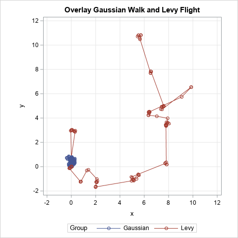
for 100 steps. You can use a SERIES plot to overlay the two paths on a single graph, as shown at the top of this article.

The graph shows that the animal that is modeled by using a Gaussian step size spends its entire time foraging near the origin.
In contrast, the animal modeled by using the truncated Levy process forages for a while near the origin, then flies away to another region.
It forages there for a while, then flies away again. This process continues. After 100 steps, the animal has explored more than a dozen different feeding sites.

Summary

A previous article discussed simulating the foraging/hunting behavior of animals by using a random sequence of Gaussian or Levy
variates to model the animal’s movements. The previous model used the SAS DATA step to perform a simulation.
This article was inspired by a similar simulation that was written by Jay Laramore in the SAS IML language.
The IML program emphasizes breaking the problem into a series of independent functions that are vectorized.
The functions can be assembled into a Gaussian simulation and a Levy simulation by changing only one line in the program.
The results of the programs demonstrate the difference between the two models of animal locomotion.

You can download the SAS IML program that simulates Levy flight and create all graphs in this article.