Calculate the Gini-Simpson diversity index in SAS

An article by David Corliss in Amstat News (Corliss D. (2025) “Quantifying Diversity:
Calculating the Gini-Simpson Diversity Index”)
discusses a new statistical measure of diversity that was adopted by the US Census Bureau.
The statistic is called the Gini-Simpson diversity index.
The Census Bureau has published an article about how to interpret the statistic and how they Bureau uses it
to estimate the racial and ethnic diversity of the US population (Jensen et al. (2021), “Measuring Racial and Ethnic Diversity for the 2020 Census”).
This blog post shows how to compute the Gini-Simpson diversity index in SAS.

The Gini-Simpson diversity index

There are two diversity statistics that are mathematically equivalent:

• The Simpson index: Suppose there are R groups.
  The Simpson index, λ, is the probability that two items selected at random from the sample belong to the same group.
  For a finite population, let N be the size of the sample and let n_i be the size of the i_th subgroup.
  Then the Simpson index, λ, is defined by
  
  
       
  \( \lambda = \sum\limits_{i=1}^R \frac{n_i}{N} \frac{n_i-1}{N-1}\)
  
• 
  The Gini-Simpson index: This statistic is defined
  as 1 – λ and estimates the probability that
  two items selected at random from the population do NOT belong to the same group.

The number of groups, R, is called the richness of the sample.
The distribution of the n_i tells you whether the groups are evenly divided.
Diversity is a measure of both richness and homogeneity.

From the definition, it is clear that if there is only one homogeneous group (R=1), then λ=1.
If there is one main group and a few relatively small groups, then λ will be close to 1.
Similarly, if each item belongs to its own group (R=N), then λ=0.
If there are many small groups and no primary group, then λ will be close to 0.

It is not hard to derive
the formula for the Simpson index, which is the probability for picking two matching items at random from the sample.
Consider the probability of drawing two items that are both from the first group. The number of observations
for Group 1 is n1, so the probability that the first item is from Group 1 is n1/N. We do not replace the first item, so there are now
n1-1 items left in Group 1 and N-1 items left in the sample. Therefore, the probability that the second item is from Group 1 is (n1-1)/(N-1).
The probability that both items are from Group 1 is the product (n1/N)*((n1-1)/(N-1)).
In a similar way, the probability that both items are from Group 2 is (n2/N)*((n2-1)/(N-1)).
Continuing this computation for all possible groups and adding the results shows that λ is the probability that both items are from the same group.
Of course, the probability that both items are from different groups is the complementary probability, 1 – λ.

Compute the Gini-Simpson diversity index in SAS

The computation of the Gini-Simpson diversity index requires that you have a vector of counts.
That is, you need the counts n_i for each subgroup, i=1,…,R.
If you have raw data, you can use PROC FREQ to count the number of observations in each subgroup and use the
OUT= option on the TABLE statement to write the frequencies to a data set, as follows:

%let RAW_DSNAME = sashelp.cars;     /* unsummarized data. Use PROC FREQ to get counts */
%let CAT_VAR = Type;                /* categorical variable to analyze */
 
title "Diversity of the &CAT_VAR Variable in the &RAW_DSNAME Data";
proc freq data=&RAW_DSNAME;
   tables &CAT_VAR / out=Summary1 nocum;
run;

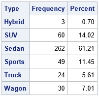
Intuitively, the TYPE variable is moderately diverse. There are N=428 observations. Of these, 262 (61%) are sedans.
If you select two observations at random from the data, it is reasonable to expect the
observations to have the same value, but the exact probability isn’t clear.
The Simpson index is the exact probability that the observations have the same value.
The Gini-Simpson index is the exact probability that the observations have different values.

The computation of these statistics requires the sum of the counts. There are several ways to get the sum,
but an easy way to compute the sum and add it as a new variable is to use PROC SQL.

After adding the sum of counts to the data, it is straightforward to write a SAS DATA step that computes the
Simpson and Gini-Simpson diversity statistics, as follows:

/* the output from PROC FREQ conatins a variable named 'Count'.
   Add the constant column 'Sum', where Sum=sum(Count) */
proc sql;
   create table Summary as
   select *, (select sum(Count) from Summary1) as Sum
   from Summary1;
quit;
 
/* compute the Simpson and Gini-Simpson statistics for &CAT_VAR */
data Diversity;
label Sum = "N"
      SimpsonIndex = "Simpson Index"           /* Prob that two items are the same type */
      GiniSimpsonIndex = "Gini-Simpson Index"; /* Prob that two items are different types */
retain SimpsonIndex 0;
set Summary end=EOF;
SimpsonIndex + (Count/Sum) * (Count-1)/(Sum-1);
GiniSimpsonIndex = 1 - SimpsonIndex;
keep Sum SimpsonIndex GiniSimpsonIndex;
if EOF then output;
run;
 
proc print data=Diversity label noobs; run;

The output shows the diversity indices for the TYPE variable in the SASHELP.CARS data set.
If you draw two observations at random, there is a 41.4% chance that they have the same values.
Similarly, there is a 58.6% chance that they have different values.

If your data are pre-summarized (that is, you already have the counts for each subgroup), you can omit the PROC FREQ
step and proceed immediately to the PROC SQL step. I leave that modification as an exercise for the reader.

A SAS macro to compute the Gini-Simpson diversity index

You can encapsulate the procedures in a SAS macro. The following macro assumes that
the data are unsummarized. You can modify the macro if you have pre-summarized counts.

%macro GiniSimpsonIndex(dsname, cat_var);
   title "Diversity in the &cat_var Variable in the &dsname Data";
   proc freq data=&RAW_DSNAME;
      tables &CAT_VAR / out=Summary1 nocum;
   run;
   /* the output from PROC FREQ conatins a variable named 'Count'.
      Add the constant column 'Sum', where Sum=sum(Count) */
   proc sql;
      create table Summary as
      select *, (select sum(Count) from Summary1) as Sum
      from Summary1;
   quit;
   /* compute the Simpson and Gini-Simpson statistics for &CAT_VAR */
   data Diversity;
   label Sum = "N"
         SimpsonIndex = "Simpson Index"           /* Prob that two items are the same type */
         GiniSimpsonIndex = "Gini-Simpson Index"; /* Prob that two items are different types */
   retain SimpsonIndex 0;
   set Summary end=EOF;
   SimpsonIndex + (Count/Sum) * (Count-1)/(Sum-1);
   GiniSimpsonIndex = 1 - SimpsonIndex;
   keep Sum SimpsonIndex GiniSimpsonIndex;
   if EOF then output;
   run;
 
   proc print data=Diversity label noobs; run;
   title;
%mend;
 
%GiniSimpsonIndex(dsname=sashelp.cars, cat_var=Type);

The output is exactly the same as before and is not shown. Now that you have a macro,
you can easily run the analysis on other data sets or other categorical variables.
Here’s another example for the ORIGIN variable, which has three levels:

%GiniSimpsonIndex(dsname=sashelp.cars, cat_var=Origin);

Notice that the frequency counts for the ORIGIN variable are roughly even. The probability that two randomly chosen observations have the same
value of origin is 33.5%.

Let’s do a sanity check by performing a quick back-of-the-envelope calculation. For the ORIGIN variable, each level contains
approximately 1/3 of the observations. Let X be a discrete uniform random variable for which P(X=’A’) = P(X=’B’) = P(X=’C’) = 1/3.
Let’s compute the probability that two random variates from X are identical. The possible outcomes are AA, AB, AC, BA, BB, BC, CA, CB, and CC,
and each event is equally likely. Therefore the probability that two consecutive draws are the same is 1/3.
This simpler computation shows why the Simpson index is approximately 33.3% for the ORIGIN variable. It also shows that
for three categories, the “most diverse” arrangement will have a Simpson index that is approximately 0.33
and a Gini-Simpson index that is approximately 0.66.

A SAS IML function to compute the Gini-Simpson diversity index

An advantage of the SAS IML language is that it can perform both row-oriented computations (like the DATA step)
and column-oriented computations (like PROC SQL). The following statements define a function in SAS IML that computes the
sum, Simpson index, and Gini-Simpson index for a vector of counts. If the data are not pre-summarized, you can use TABULATE subroutine
to compute the frequencies for each level of a categorical variable, as follows:

proc iml;
/* Compute the Gini-Simpson diversity index
   Input: Vector of counts (n1, n2, ..., nR) 
   Output: a 1x3 vector. The elements are:
           N : sum of counts
           Simpson index of homogeneity
           Gini-Simpson index of diversity   
*/
start GiniSimpsonIndex(count);
   Sum = sum(count);
   SimpsonIndex = sum( (count/Sum) # ((count-1)/(Sum-1)) );
   GiniSimpsonIndex = 1 - SimpsonIndex;
   return Sum || SimpsonIndex || GiniSimpsonIndex;
finish;
 
use sashelp.cars; read all var {"Type"}; close;
call tabulate(Levels, count, Type);
print count[c=Levels];
 
r = GiniSimpsonIndex(count);
labls = {"N" "Simpson Index" "Gini-Simpson Index"};
print r[L="" c=labls F=BEST7.];

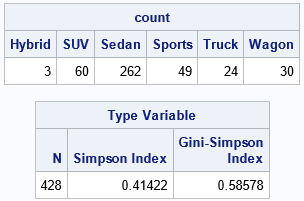
The IML function only needs three statements to compute the statistics, but it produces
the same output as Base SAS calls to PROC FREQ, PROC SQL, and the DATA step.
In IML, you can easily specify the vector of counts directly. For example, the following
statements specify the frequencies of the ORIGIN variable in the SASHELP.CARS data:

count = {158, 123, 147};
r = GiniSimpsonIndex(count);
print r[L="" c=labls F=BEST7.];

Summary

The US Census Bureau uses the Gini-Simpson index as a measure of diversity.
The Gini-Simpson index is the probability that two items (chosen at random from the sample) are different types.
Equivalently, the Simpson index is a measure of homogeneity.
It is the probability that two randomly chosen items are the same type.
This blog post shows how to compute the Simpson and Gini-Simpson diversity index in SAS.
You can use either Base SAS to define a macro, or you can implement a function in SAS IML.
The macro in this article is for unsummarized (raw) data, but can be modified to support pre-summarized counts.