A historical method of generating random normal variates

Decades ago, it was a challenge to generate (pseudo-) random numbers that had good statistical properties.
The proliferation of desktop computers in the 1980s and ’90s led to many advances in computational mathematics,
including better ways to generate pseudorandom variates from a wide range of probability distributions. (For brevity, I will drop the “pseudo-” prefix.)

Today, it is trivial to simulate high-quality random variates from a probability distribution
such as the standard normal distribution.
But that was not always the case. Early software libraries
might be able to generate a uniform random variate in the interval (0,1), but often did not
support other probability distributions. In those days, simulating normal random variates could be a challenge.

One algorithm used the sum of 12 random uniform variates to approximate the standard normal distribution.
Although this method has been replaced by more accurate methods (see the Appendix),
it is fun to revisit the older method and marvel at its simplicity and accuracy. (Spoiler: The number 12 is used for a reason!)

The Irwin-Hall distribution

In 1927, Oscar Irwin and Philip Hall independently published papers about the
distribution of the sum of n independent random uniform variates.
Today, the distribution is called the Irwin-Hall distribution, or sometimes the uniform-sum distribution.
The Wikipedia article
about the Irwin-Hall distribution gives the exact PDF of the sum of n uniform variates. The support of the distribution is [0, n].
The uniform-sum has the following moments:

• Mean: n / 2
• Variance: n / 12
• Skewness: The distribution is symmetric, so the skewness is 0.
• Excess kurtosis: -6 / 5n

As n increases, the Central Limit Theorem (CLT) ensures that the distribution approaches a normal distribution
with the mean and variance given by the preceding formulas. Visual inspection (see the Wikipedia article) indicates that the
distribution looks normal for n ≥ 8.

Look at the formulas when n = 12. The mean of the distribution is 6, the variance is 1, the skewness is 0, and the kurtosis is -0.1, which is small.
If we center the distribution by subtracting 6, we obtain moments that are close to the moments of the standard normal distribution.
Both distributions have mean=0, var=1, and skew=0.
Only the kurtosis is different.
The kurtosis of the normal distribution is 0, whereas the kurtosis of the uniform-sum distribution is slightly negative, which means that the
uniform-sum distribution has less mass in its tails.
Notice that the support of the (centered) uniform-sum distribution is [-6,6], whereas the standard normal distribution has infinite support.

Because of the CLT and the moments, you can use the (centered) uniform-sum distribution when n = 12 to approximate the standard normal distribution.
This is simple to program and was used by early researchers who did not have access to more sophisticated methods
for generating random normal variates.

Simulate from the Irwin-Hall distribution in SAS

Let’s simulate from the Irwin-hall distribution and see whether the distribution of the variates approximate the standard normal distribution.
However, I want to emphasize that this is NOT a modern method!
If you want to generate a standard normal variate in SAS, you can simply use the RAND(“Normal”) call directly, as shown in the Appendix.

The following DATA step program implements generating random variates from the (centered) uniform-sum distribution when n = 12.
The program simulates 12 uniform random variates and computes their sum. It then subtracts 6, which is the expected value of the sum.
The program then calls PROC UNIVARIATE in SAS to analyze the resulting distribution.

%let nIH = 12;  /* sum this many uniform variates in the Irwin-Hall distribution */
%let N = 10000;
data IrwinHall;
call streaminit(12345);
EsumU = 0.5 * &nIH;    /* expected value (mean) of the sum of 12 U ~ U(0,1) */
do i = 1 to &N;
   sum = 0;
   do k = 1 to &nIH;
      sum + rand("Uniform");
   end;
   x = sum - EsumU;
   output;
end;
keep x;
run;
 
proc univariate data=IrwinHall;
   var x;
   histogram x / normal(mu=0 sigma=1)   /* overlay PDF for N(0,1) */
                 midpoints=(-4 to 4 by 0.5) odstitle="(Sum of 12 Uniform Variates) - 6";
   ods select Moments Histogram GoodnessOfFit;
run;

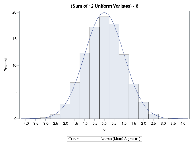
The histogram shows the distribution of 10,000 random variates from the Irwin-Hall distribution.
The graph overlays the PDF of a standard normal distribution. The fit is very good.
To the eye, the Irwin-Hall variates look very much like a normal distribution.

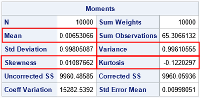
The sample moments of the Irwin-Hall variates are also in accordance with what you would expect from normal variates.
The sample mean, variance, skewness, and kurtosis are not very far away from the expected values of 0, 1, 0, and 0, respectively.
(The expected kurtosis is -0.1, not 0.)

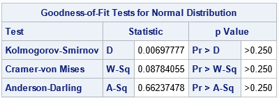
Lastly, when you tell PROC UNIVARIATE to overlay the standard normal distribution, that causes the procedure to run
several goodness-of-fit tests for the data. All p-values are large, which means that we cannot reject
the null hypothesis that the data are from a standard normal distribution.

Why n=12?

In case it wasn’t clear, when n=12 uniform variates are summed, the variance of sum is 1.
You could use higher value of n, which would make the kurtosis would be even closer to 0.
However, the variance of the Irwin-Hall distribution is
n/12, so you would need to scale the resulting distribution by 12/n before using it.
For practical purposes, n=12 is a convenient value that is fast, needs no adjustments, and results in a distribution
that is close to the normal distribution.

Summary

Early researchers in computational statistics did not have access to the many tools that are available today.
Sometimes, numerical libraries did not provide a function for generating random variates from a standard normal distribution.
However, the early researchers cleverly noticed that they could approximate random normal variates if
they used the sum of 12 uniform random variates (and subtracted 6). This article shows how simple it is to implement the sum-of-12 algorithm. Furthermore,
it shows that the resulting variates (from the Irwin-Hall distribution) are indeed a good approximation to random normal variates.

Modern software provides better methods for simulating normal variates, but it is fun to look back at early algorithms and
realize that they were rather good at approximating normality despite their simplicity.

Appendix: Generating random normal variates in SAS

To generate random standard normal variates in SAS, you can use the RAND(“Normal”) call.
Internally, SAS uses the Marsaglia
and Bray (1964) “polar method” for generating random normal variates.

%let N = 10000;
data Normal;
call streaminit(12345);
do i = 1 to &N;
   x = rand("Normal");
   output;
end;
keep x;
run;
 
proc univariate data=Normal;
   var x;
   histogram x / normal(mu=0 sigma=1) odstitle="&N Normal Variates";
   ods select Moments Histogram GoodnessOfFit;
run;